

The term theoretical chemistry or computational chemistry may be defined as the mathematical description of chemistry. The term computational chemistry is generally used when a mathematical method is sufficiently well-developed to be automated for implementation on a computer. Very few chemistry aspects can be computed exactly, but almost every aspect of chemistry has been described in a qualitative or approximately quantitative computational scheme. However valuable this aspect is, we often use constructs that do not fit in the scientific method scheme as it is typically described. One of the most commonly used constructs is a model. A model is a simple way of describing and predicting scientific results, which is an incorrect or incomplete description. But before going deep into different models, we will see some terms and definitions associated with these computational calculations. Potential Energy Surface and Saddle Point, these two terms will come to one’s mind first, as soon as one enters these computational chemistry calculations. However, one can say these two terms are the two sides of a coin. PES and Saddle Point both are very much crucial in understanding the reaction transition states and reaction pathways.
Potential Energy Surface (PES):
The potential energy surface (PES) is a central concept in computational chemistry. A Potential Energy Surface (PES) describes the potential energy of a system, especially a collection of atoms, in terms of specific parameters, usually the atoms’ positions. The surface might define the energy as a function of one or more coordinates; if there is only one coordinate, the surface is called a potential energy curve or energy profile. The Born–Oppenheimer approximation says that the nuclei are essentially stationary in a molecule compared to the electrons. This is one of the cornerstones of computational chemistry because it makes the concept of molecular shape (geometry) meaningful, makes possible the concept of PES, and simplifies the application of the Schrödinger equation to molecules by allowing us to focus on the electronic energy and add in the nuclear repulsion energy. PES helps us to explain Geometry optimisation and Transition State optimisation. Now, some details about PES are described below —
The dimension of PES:
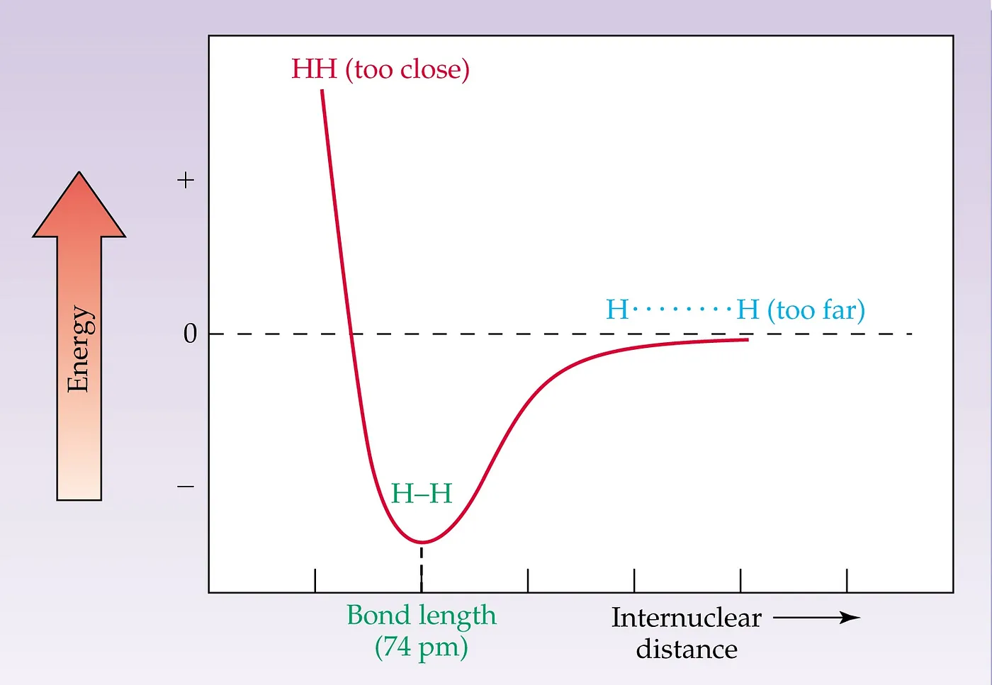
Figure 1: 1D PES Diagram for Diatomic Molecule
The most straightforward PES diagram is like the above (Figure 1), i.e. 1D PES Diagram. It is for the bond stretch of a simple diatomic molecule. At the minima of the curve, the interacting repulsion energy will be the least, which is the bond length in the ground state. This is more correctly known as the equilibrium bond length because thermal motion causes the two atoms to vibrate about this distance. Now, we can find that the interaction between particles is going to be smaller and smaller if we go to the right side of the minima along the X-direction. In the infinity, the two molecules stop interacting. Whereas, if we consider going to the left side from the minima along the X-axis, we can find that the system’s overall energy is increasing exponentially, leading to infinite energy.
But all PES diagram is not that much simple. The most important thing is in the practical field, we mainly deal with a multi-dimensional PES diagram. The following process measures the dimension of the PES diagram —
To define an atom’s location in 3-dimensional space requires three coordinates (e.g., xx, yy, and zz or rr, θθ and ΦΦ in Cartesian and Spherical coordinates) or degrees of freedom. However, a reaction and hence the corresponding PES do not depend on the absolute position of the reaction, only the relative positions (internal degrees). Hence both translation and rotation of the entire system can be removed (each with 3 degrees of freedom, assuming non-linear geometries). So the dimensionality of a PES is 3N−6 where N is the number of atoms involves in the reaction, i.e., the number of atoms in each reactant). The PES is a hypersurface with many degrees of freedom and typically only a few are plotted at any one time for understanding.
So, we should have drawn a 4D PES diagram to plot a molecule and its energy accordingly. But for simplicity, we take a 2D slice (the energy is the third coordinate) of a molecule with 3 degrees of freedom; It is the bond angle held fixed that defines the slice. You can see how these types of slices are drawn in the diagram in Figure 2 —
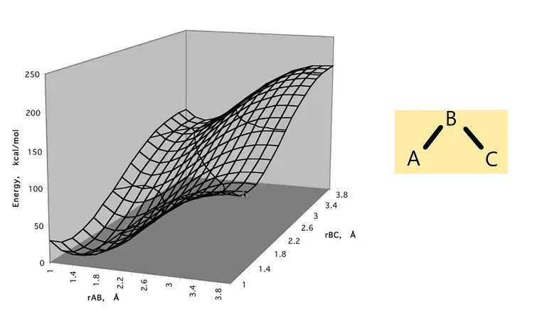
Figure 2: Slice of a PES diagram
In the above diagram, one can change another one to get the specific energy on that particular position in fixing one bond length.
Mathematical Definition:
A set of atoms’ geometry can be described by a vector, r, whose elements represent the atom positions. The vector r could be the set of the atoms’ Cartesian coordinates or could also be a set of inter-atomic distances and angles. Given r, the energy as a function of the positions, V(r), is the value of V(r) for all values of r of interest. Using the landscape analogy from the introduction, V(r) gives the height on the “energy landscape” so that the concept of a potential energy surface arises.
Stationary Points and Saddle Point:
Saddle point and stationary points all lie on the slice of PES. But these terms are not equivalent. Mostly, in our computational calculations, we give more preferences to the saddle point than stationary points. Let’s have a look at what these are —
Stationary Points:
In mathematics, particularly in calculus, a stationary point of a differentiable function of one variable is a point on the graph of the function where the function’s derivative is zero; for the PES diagram, stationary points are the same in meaning. Stationary points in the PES diagram indicate that the energies are minimum corresponding to physically stable chemical species. For example, the 4 SP points in Figure 3 are four stationary points in that PES diagram.
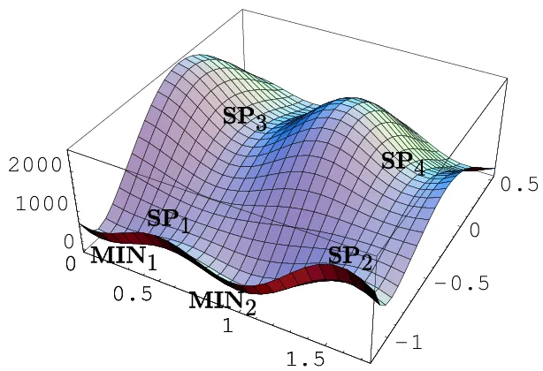
Figure 3: Stationary Points in PES
Saddle Point
The reaction path is defined as the pathway between the two minima. The reactant passes through a maximum in energy along the reaction pathway, connecting the two minima. That maxima is called a saddle point. While this point is a maximum along the minimum energy path in the two valleys, this is a minimum point if we traverse a path in a plane perpendicular to the minimum energy path at the saddle point. The Transition State is the most cultured area for a chemical reaction. A transition state is a first-order saddle point on a potential energy surface (PES). Transition-state energies can be close to excited states. This often implies that the usual MO-based computational methods may not be as accurate for transition states as for minima on a PES. A better image for saddle point and transition state is shown in Figure 4.
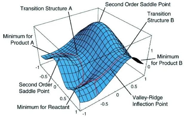
Figure 4: Saddle Point and Transition State
Example:
- • Suppose we have a molecule with more than one geometric parameter, for example, water: the geometry is defined by two bond lengths and a bond angle. If we reasonably content ourselves with allowing the two bond lengths to be the same, i.e. if we limit ourselves to C₂ᵥ symmetry (two planes of symmetry and a two-fold symmetry axis), then the PES for this triatomic molecule is a graph of E versus two geometric parameters, q1 = the O–H bond length, and q2 = the H–O–H bond angle (fig.-1.5). Figure 1.5 represents a two dimensional PES (a regular surface is a 2-D object) in the three-dimensional graph; we could make an actual 3-D model of this drawing of a 3-D diagram of E versus q1 and q2.
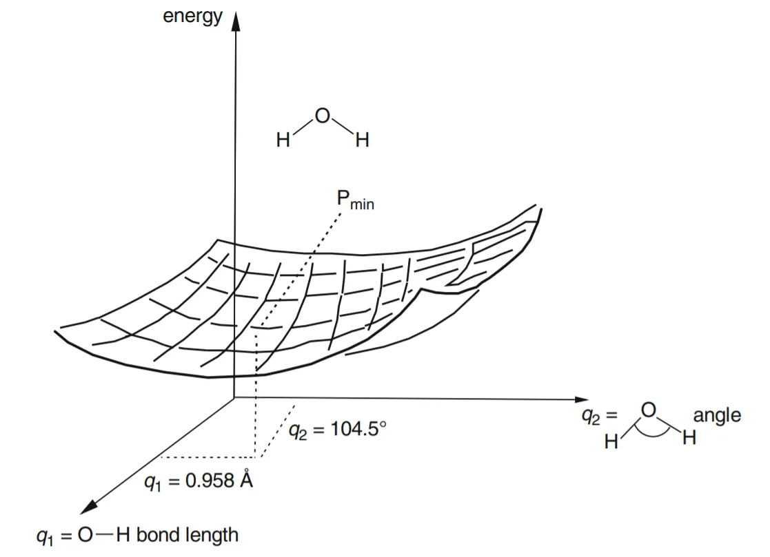
Figure 5: The H₂O potential energy surface. The point Pₘᵢₙ corresponds to the minimum-energy geometry for the three atoms, i.e. to the water molecule’s equilibrium geometry.
- • We can go beyond water and consider a triatomic molecule of lower symmetry, such as HOF, hypofluorous acid. This has three geometric parameters, the H–O and O–F lengths and the H–O–F angle. To construct a Cartesian PES graph for HOF analogous to that for H2O would require us to plot E vs q1 = H–O, q2 = O–F, and q3 = angle H–O–F. We would need four mutually perpendicular axes for E, q1, q2, q3 (fig.-1.6). Since such a four-dimensional graph cannot be constructed in our three-dimensional space, we cannot accurately draw it. The HOF PES is a 3-D “surface” of more than two dimensions in 4-D space: it is a hypersurface, and potential energy surfaces are sometimes called potential energy hypersurfaces. Despite the problem of drawing a hypersurface, we can define the equation E = f (q1, q2, q3) as the potential energy surface for HOF, where f is the function that describes how E varies with the q’s, and treat the hypersurface mathematically.
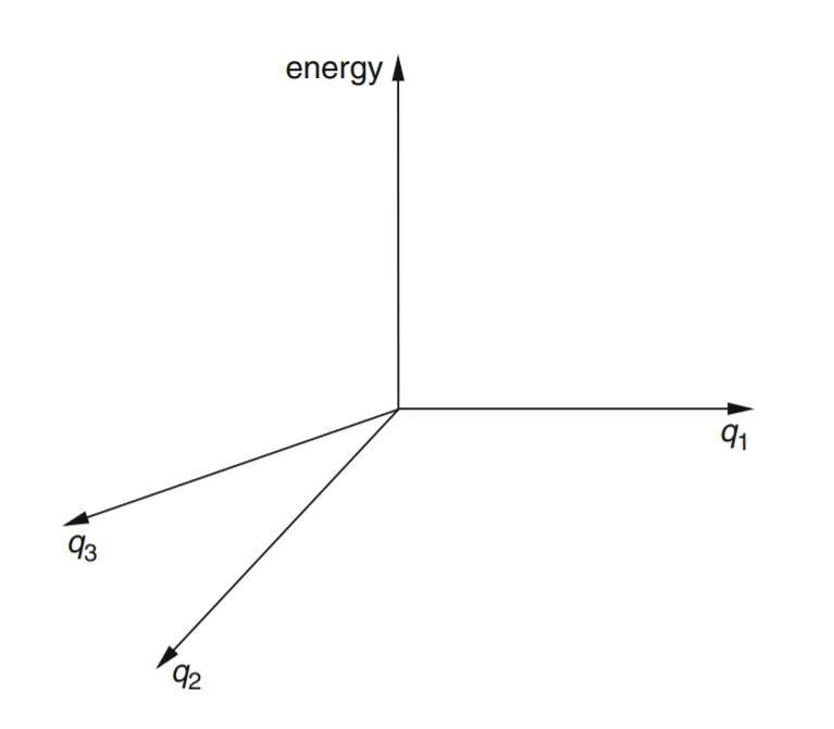
Figure 6: We would need four mutually perpendicular axes to plot energy against three geometric parameters in a Cartesian coordinate system. Such a coordinate system cannot be constructed in our three-dimensional space. However, we can work with such coordinate systems and the potential energy surfaces in them mathematically.
Equilibrium Constant and Rate Constant Calculation:
Now, PES does not show kinetic energy! So, everyone’s favourite picture of a dynamic molecule being a ball rolling on the surface is misleading if you think of the energy decreasing as you go downhill. It doesn’t make any sense to roll over a ball as many times the number of molecules and to see which one is crossing the TS energy and which is not. So, we change our aspect of viewing somewhat to calculate our Equilibrium Constant and Rate Constant. We switch our coordinate of Energy to Free Energy, i.e. G(marked in Figure 7(2) using red colour). If we cut the PES perpendicularly of the screen and along the dotted direction line of the diagram of Figure 7(1), folded out to make it flat and see the cross-sectional diagram, we’ll get a diagram like Figure 7(2).
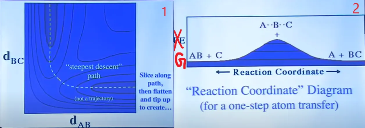
Figure 7: PES cross-sectional diagram without cutting (1) and after cutting (2).
Now, we can easily get ΔG for individual two species (out of reactant, Transition State, and product). Hence, we can calculate the Equilibrium Constant and Rate Constant for a specific reaction pathway using Eyring’s Transition State Theory(Figure 8).
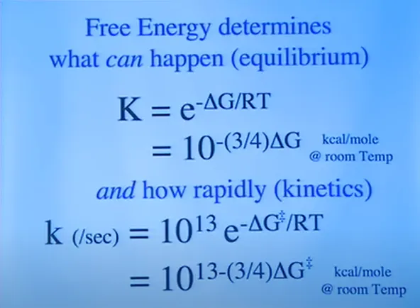
Figure 8: Equations for calculating Equilibrium Constant and Rate Constant from Eyring’s Transition State Theory [Where K is the Equilibrium Constant, and k is the Rate Constant(per second).
References:
• Computational Chemistry by Errol G. Lewars (2nd Edition)
• Chemical Kinetics Chapter of UCD Chem 107B: Physical Chemistry for Life Scientists
• Computational Chemistry by Chris Cramer
• Wikipedia
• Professor McBride’s web resources for CHEM 125 (Lecture 37)
⁕ ⁕ ⁕